Carbon emissions calculation
HEAT assesses the carbon emissions associated with changes in walking and cycling in three main steps (1):
- Estimating the shift from motorized travel to walking or cycling;
- Calculating the carbon emissions associated with the motorized travel that is replaced; and
- Estimating the economic value of the change in carbon emissions.
Step 1: Estimating the shift from motorized travel
In two-case assessments, such as comparing before and after an intervention, HEAT can estimate how much walking and/or cycling replaces motorized travel. Users are asked to adjust their walking and cycling data to account for three factors:
- Reassigned or induced travel: Walking or cycling that has simply shifted to a different route or destination, or represents new travel, does not replace motorized travel and is therefore excluded from the carbon assessment.
- Recreational travel: Walking and cycling for recreation are assumed not to replace motorized travel and are therefore excluded.
- Travel shifted from other modes: The remaining walking and cycling is assumed to replace other modes of transport. HEAT provides default diversion rates, which users can modify, to estimate the share shifted from car, public transport and other modes when direct data are not available (see diversion rates below).
For example, if 5% of cycling on a new route has been reassigned from another route and another 5% represents newly induced travel, 90% of the cycling volume is considered relevant for the carbon assessment.
In a single-case assessment, which assumes a steady-state situation, reassigned and induced walking and cycling are excluded by definition. The proportions attributed to other modes are used to estimate how much motorized travel would otherwise have taken place. The same approach is used in a two-case assessment when the user selects “no data” for motorized modes.
Diversion rates
Carbon module: guidance on “mode shift” and “diversion rates” (step 1)
What are diversion rates? How is mode shift handled in the carbon module?
The carbon tool excludes new trips that do not displace trips done previously by motorized modes from an assessment of carbon emissions from motorized travel. This has been implemented by parameterizing so-called “diversion rates” [1] for walking and cycling for transport, with values between 0 and 1 for the shares of new cycling (or walking) that is estimated to be shifted from motorised travel and walking (or cycling). The motorised modes considered include car (as driver or passenger), local bus, urban rail (incl. tram, underground) and motorcycle (not shown separately in Figure 1 for space reasons). For intervention assessments, the user will be asked to consider excluding any induced (entirely new trips not replacing motorized travel) or reassigned (route shift rather than mode shift) travel activity. The diversion rates are applied to the volume of walking and/or cycling entered by the user.
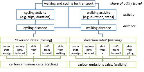
Note: the dashed boxes are only really relevant for assessments of ‘before’ vs. ‘after’ comparisons.
An example
Assume an infrastructure intervention has led to an increase in connectivity, making it easier/safer to travel via the new route. ‘New’ cycling trips are being recorded along that route (e.g. using trip counters or user intercept surveys). Some of the new trips were done previously using different modes (mode shift), while some were on a parallel route that perhaps wasn’t as convenient or safe to use (route shift, or route reassignment). Some even did not exist at all before the intervention (newly generated or induced demand that was suppressed before). The carbon module will focus on the former (mode shift) and not take into account the latter (route shift, newly induced trips).
Changeable default values
For the diversion rates of the remaining volume of walking or cycling, HEAT provides recommended values based on a conservative assessment of the evidence found in the appraisal guidance [1], project evaluation [2-5] and impact scenario [6-8] literatures.
For example, UK transport appraisal guidance (WebTAG) [1] and Mulley et al [9] reported car substitution rates of 25% to 30%. ECF [10] suggested to use: car 32%, bus 42% and walking 26%, based on mode substitution rates observed for bicycle trips of bicycle share schemes.
The HEAT recommended default values for diversion rates from other transport modes to cycling or walking are:
| From: | To: walking | To: cycling | To: e-biking |
|---|---|---|---|
| Driving | 20% | 30% | 30% |
| Public transport | 60% | 50% | 30% |
| Walking | — | 20% | 10% |
| Cycling | 20% | — | 30% |
| From: | To: walking | To: cycling | To: e-biking |
|---|---|---|---|
| Car or van (as driver or passenger) | 20% | 30% | 30% |
| Local bus | 50% | 30% | 10% |
| Urban rail (light rail, trams, metro) | 10% | 10% | 10% |
| Train | 0% | 10% | 10% |
| Walking | — | 20% | 10% |
| Cycling | 20% | — | 30% |
Sources
1. DfT. Transport analysis guidance: WebTAG, https://www.gov.uk/guidance/transport-analysis-guidance-webtag. 2014.
2. Dons, E., et al., Physical Activity through Sustainable Transport Approaches (PASTA): protocol for a multi-centre, longitudinal study. BMC Public Health, 2015. 15: p. 1126.
3. Brand, C., A. Goodman, and D. Ogilvie, Evaluating the impacts of new walking and cycling infrastructure on carbon dioxide emissions from motorized travel: A controlled longitudinal study. Applied Energy, 2014. 128(0): p. 284-295.
4. Goodman, A., S. Sahlqvist, and D. Ogilvie, Do new walking and cycling routes increase physical activity? One- and two-year findings from the UK iConnect study. Am J Public Health, 2014. 104.
5. European Commission, OBIS (Optimising Bike Sharing in European Cities), Final Report. 2011, Brussels: European Commission.
6. Woodcock, J., et al., Public health benefits of strategies to reduce greenhouse-gas emissions: urban land transport. The Lancet, 2009. 374.
7. Keogh-Brown, M., et al., A whole-economy model of the health co-benefits of strategies to reduce greenhouse gas emissions in the UK. The Lancet, 2012. 380, Supplement 3(0): p. S52.
8. Buekers, J., et al., Health impact model for modal shift from car use to cycling or walking in Flanders: application to two bicycle highways. Journal of Transport & Health, 2015. 2(4): p. 549-562.
9. Mulley, C., et al., Valuing active travel: Including the health benefits of sustainable transport in transportation appraisal frameworks. Research in Transportation Business & Management, 2013. 7(0): p. 27-34.
10. ECF, Cycle more Often 2 cool down the planet! – Quantifying CO2 savings of Cycling. 2011, European Cyclists’ Federation (ECF): Brussels.
Step 2: Calculating carbon emissions
The second step converts the estimated replacement of motorized travel into carbon emissions avoided or saved.
HEAT considers three types of emissions:
- operational emissions: emissions produced while vehicles are being used. These include country- and year-specific information on average trip lengths, fuel types, vehicle fleets, temperature and cold-start emissions, as well as a user-adjustable assumption about traffic conditions.
- energy supply emissions: emissions associated with producing and supplying the energy used for transport, including fuels such as petrol and diesel and electricity.
- vehicle lifecycle emissions: emissions associated with producing vehicles, including the materials and energy used in vehicle manufacturing.
Operational emissions
Operational emissions
Operational carbon emissions are derived by breaking carbon emissions down into changes in travel activity or travel demand (in passenger-kilometres by mode of travel – see step 1), differences in energy efficiency of each mode of travel (in megajoules per passenger-km, by mode and fuel type), and differences in carbon intensity (CO2e/MJ, by mode and fuel type) of the energy used. This represents a typical carbon emissions ‘decomposition approach’ illustrated below:
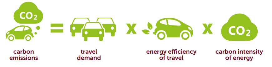
HEAT considers the effects of three contextual factors on carbon emission factors:
- distance travelled and average trip lengths;
- average speed, representing various traffic conditions in the study area; and
- mode characteristics such as vehicle type and fuel type.
For cars, HEAT considers average traffic speeds, vehicle fleet composition and the effect of ‘real-world’ driving (adding 21.6% to the carbon emissions derived from official laboratory test data; value based on the conversion factors used in the United Kingdom [1]) in the study area to calculate the amount of CO2e emitted per km when the engine is at operating temperature. This is based on published relationships between fuel consumption, average speed and conversion to carbon emissions using a standard carbon balance method. For motorcycle, bus and rail, only fuel type shares are considered, with average emission factors based on the conversion factors taken from [1]. For most countries and cities, buses are still largely powered by diesel, motorcycles are generally running almost 100% on gasoline, and urban rail is assumed to be all electric. For cars, excess emissions from cold starts (for the initial, ‘cold’ part of a journey, typically the first 3.4 km after starting) are added to this. For detailed formulas see Methods and user guide booklet (section 3.13.3 Operational emissions, p. 56-57).
Vehicle fuel type shares and average occupancy rates for each country are based on international databases, including the GAINS (Greenhouse gas–Air pollution Interactions and Synergies) model projections (IEA World Energy Outlook 2016 ‘6DS’ scenario) of the International Institute for Applied Systems Analysis for many countries and years up to 2050 [3-8]. Future projections of carbon emissions factors are thus based on available scenario data, not forecasts, therefore any projections beyond the 10-year timeframe should be treated with caution.
For cars, the user can choose between five generic traffic conditions based on typical road speeds observed in countries and cities around the world [9], including average speeds (all values in kilometres per hour) in “little or no congestion, nearly ‘free flow’” (Canberra peak 46, Vienna off-peak 45, Memphis peak 59, Paris off-peak 53); “some heavy traffic and peak time congestion” (Vienna peak 29, Curitiba off-peak 31, Bogota off peak 25); and “heavy congestion most days” (Curitiba peak 23, Prague peak 25, Paris peak 25, Berlin peak 23, Bogota peak 17, Rio de Janeiro peak 26) [9-11]. The five traffic categories are:
- Global average, urban / inner city (~32 km/h) – changeable default value;
- Little or no congestion, urban (“free flow”) (~45 km/h);
- Some peak time congestion (commute, school run), urban (~35 km/h);
- Heavy congestion most days (am, pm and inter peak), urban (~20 km/h);
- Global average, rural / inter-urban (~60 km/h).
HEAT uses country and year specific emissions factors. Table 1 provides an example for India in 2019. Other country-year combinations are available on request.
| Example: India, year 2019 | Average traffic conditions | ||||
|---|---|---|---|---|---|
| Average emissions factors, operational (gCO2e/passenger-km) | ‘Global’ average, urban | Little or no congestion (‘free flow’) | Some peak time congestion | Heavy congestion most days | Global average, rural |
| Car or van 1,2 | 126 | 110 | 121 | 156 | 103 |
| Local bus 1,2 | 81 | — | — | — | — |
| Urban rail, trams, metro (100% electric) 2 | 0 | — | — | — | — |
| Motorcycle 1,2 | 76 | — | — | — | — |
| E-bike / bicycle | 0 / 0 | — | — | — | — |
| Average ‘cold start’ emissions per trip (gCO2e/passenger-trip) 3 | |||||
| Car or van 1,2 | 52 | 45 | 50 | 64 | 42 |
Notes: (1) Takes into account weighted fuel/engine type shares for each mode, e.g. for cars in India in 2019 (44% petrol, 55% diesel, 1% electric), bus (98% diesel), motorcycle (99.5% gasoline). (2) Car occupancy rate of 1.5 (all trip purposes), local bus 14.3, average urban rail 120, motorcycle 1.05. (3) With cold/hot ratio of 1.2 and cold trip distance of 2.2 km, derived from ambient temperature of 25 degrees C and average trip length of 8 km. ‘—’ not applicable.
Sources: hot and cold emissions factor coefficients [2, 12]; vehicle fleets [3, 8], speeds [9-11].
Sources
1. DEFRA/DECC, UK Government conversion factors for Company Reporting, full 2016 dataset. 2016, Department for the Environment, Food and Rural Affairs and Department for Energy and Climate Change: London.
2. EEA, COPERT 4 (COmputer Programme to calculate Emissions from Road Transport), last accessed at http://emisia.com/content/copert-documentation on 20/02/2018. 2012, European Environment Agency: Copenhagen.
3. ACEA/ANFAC, European Motor Vehicle Parc 2014: Vehicles in Use (2009-2014). 2014, Madrid: ANFAC/ACEA.
4. SMMT, New Car CO2 Report 2014: The 13th report. 2014, London: The Society of Motor Manufacturers and Traders (SMMT).
5. IEA, World energy outlook 2015. 2015, Paris: International Energy Agency (IEA).
6. Eurostat, Transport data database, October 2015 update. Last accessed at http://ec.europa.eu/eurostat/web/transport/data/database on 10/03/2017. 2016, Brussels: Eurostat, European Commission.
7. IIASA, IIASA GAINS model, scenario WPE_2014_CLE: the updated ‘current legislation’ (after the bilateral consultations in 2014) of the PRIMES 2013 REFERENCE activity projection. 2014, IIASA: Laxenburg, Austria.
8. IIASA, IIASA GAINS model, scenario ‘6DS’ for IEA World Energy Outlook, available for Europe (for 48 countries), Asia, with separate implementations for China (31 provinces and India (15 States), and for Annex I countries of the UNFCCC Convention. Accessed at https://gains.iiasa.ac.at/models/gains_models3.html in July 2019. 2016, IIASA: Laxenburg, Austria.
9. INRIX, Global Traffic Scorecard, accessed at http://inrix.com/scorecard/ on 05/11/2019. 2018, INRIX.
10. Olson, P. and K. Nolan, In Depth: Europe’s Most Congested Cities, last accessed at https://www.forbes.com/2008/04/21/europe-commute-congestion-forbeslife-cx_po_0421congestion_slide.html on 10/02/2017. Based on INRIX data., in Forbes. 2008.
11. Newman, P. and J. Kenworthy, Sustainability and Cities: Overcoming Automobile Dependence. 1999, Washington, DC: Island Press.
12. EMEP/EEA, EMEP/EEA air pollutant emission inventory guidebook 2016, Technical guidance to prepare national emission inventories. 2016, European Environment Agency: Copenhagen.
Energy supply emissions
Carbon emissions (step 2)
Energy Supply Emissions
Carbon emissions from energy supply include upstream emissions from the extraction, production, generation and distribution of energy supply, including fossil and electric fuels to power cars, buses and trains. The adopted approach uses ‘well-to-tank’ (WTT) emissions factors for different energy supply pathways for transport fuels (gasoline, diesel, electricity, etc.) [1], taken from published and well respected sources including the JEC Well-to-Wheels (WTW) study [2] and its use in developing national recommended values [3]. For e-bikes, cars, buses, urban rail, this is based on different WTT values for gasoline (0.654 kgCO2e per kg of fuel), diesel (0.688 kgCO2e per kg of fuel) and delivered electricity[1] (e.g. for India this is a relatively high 1.64 kgCO2e in 2019, due to the high share of coal generation). As with operational emissions, an uplift of 21.6% was applied to account for ‘real world’ driving conditions. Note the electricity factors vary significantly between countries (up to 3 orders of magnitude, reflecting the use of high shares of renewable sources vs. high shares of fossil fuels); therefore, the tool is using country specific factors that were based on the widest possible country comparison from an authoritative source [4]. An example for India in 2019 is given in Table 1.
| Example: India, year 2019 | Average traffic conditions | ||||
|---|---|---|---|---|---|
| Average emissions factors, energy supply (gCO2e/passenger-km) | Global average, urban | Little or no congestion (‘free flow’) | Some peak time congestion | Heavy congestion most days | Global average, rural |
| Car or van 1,2 | 28 | 25 | 27 | 35 | 23 |
| Local bus 1,2 | 21 | — | — | — | — |
| Urban rail, trams, metro (100% electric) 2 | 63 | — | — | — | — |
| Motorcycle 1,2 | 17 | — | — | — | — |
| E-bike / bicycle | 16 / 0 | — | — | — | — |
Main sources: well-to-tank emissions factors [2, 3]; electricity emissions factors [4]; vehicle fuel shares [5].
Sources
1. Odeh, N., N. Hill, and D. Forster, Current and Future Lifecycle Emissions of Key „Low Carbon‟ Technologies and Alternatives, Final Report. 2013, Harwell, UK: Ricardo AEA for the Committee on Climate Change.
2. JEC, JEC Well-To-Wheels Analysis, Report EUR 26237 EN – 2014. Last accessed at http://iet.jrc.ec.europa.eu/about-jec/sites/iet.jrc.ec.europa.eu.about-jec/files/documents/report_2014/wtt_report_v4a.pdf on 10/03/2017. 2014, Brussels: JEC – Joint Research Centre-EUCAR-CONCAWE collaboration.
3. DEFRA/DECC, UK Government conversion factors for Company Reporting, full 2016 dataset. 2016, Department for the Environment, Food and Rural Affairs and Department for Energy and Climate Change: London.
4. Ecometrica, Electricity-specific emission factors for grid electricity. 2011: Ecometrica.
5. IIASA, IIASA GAINS model, scenario ‘6DS’ for IEA World Energy Outlook, available for Europe (for 48 countries), Asia, with separate implementations for China (31 provinces and India (15 States), and for Annex I countries of the UNFCCC Convention. Accessed at https://gains.iiasa.ac.at/models/gains_models3.html in July 2019. 2016, IIASA: Laxenburg, Austria.
[1] This includes emissions from electricity generation and its transport and distribution (T&D) and from the generation well-to-tank and T&D well-to-tank stages.
Vehicle lifecycle emissions
HEAT considers lifecycle carbon emissions from the manufacture of vehicles (the clear majority of vehicle life-cycle carbon emissions, apart from operational ones), with aggregate carbon values per vehicle type (cars, motorcycles, bikes and public transport vehicles) derived assuming typical lifetime mileages, mass body weights, material decomposition and material-specific emission and energy use factors.
The key inputs, assumptions and derived carbon emissions factors per passenger-km are shown for India in Table 1. The HEAT tool uses time independent but country-specific factors, reflecting local differences in occupancy rates for the different motorized modes [1].
| Mode | Total vehicle weight (tonnes) | CO2e per vehicle (tCO2e/veh.) | Lifetime mileage (km) | CO2e per pass-km (gCO2e/pkm) (*) |
|---|---|---|---|---|
| Bicycle | 0.017 | 0.10 | 20,000 | 4.9 |
| E-bike / pedelec ($) | 0.024 | 0.19 | 20,000 | 9.3 |
| Motorcycles | 0.15 | 0.54 | 50,000 | 10.3 |
| Average car (~1% El. vehicles) | 1.295 | 4.7 | 150,000 | 20.7 |
| Average bus | 11 | 39.5 | 1,000,000 | 2.8 |
| Urban rail | 66 | 237.1 | 1,500,000 | 1.3 |
($) battery and motor add 7kg in weight; assumed 2.5 gCO2e/km for the battery based on [2].
(*) Car occupancy rate of 1.5 (all trip purposes), local bus 14.3, average urban rail 120, motorcycle 1.05.
Sources: lifecycle data [2]; electricity emissions factors [3]; vehicle fuel shares [4]; load factors [1].
Sources
1. EC DG Climate Action, Transport database TRACCS (Transport data collection supporting the quantitative analysis of measures relating to transport and climate change). 2013, Brussels: Emisia, Infras and IVL for the European Commission.
2. Odeh, N., N. Hill, and D. Forster, Current and Future Lifecycle Emissions of Key „Low Carbon‟ Technologies and Alternatives, Final Report. 2013, Harwell, UK: Ricardo AEA for the Committee on Climate Change.
3. Ecometrica, Electricity-specific emission factors for grid electricity. 2011: Ecometrica.
4. IIASA, IIASA GAINS model, scenario ‘6DS’ for IEA World Energy Outlook, available for Europe (for 48 countries), Asia, with separate implementations for China (31 provinces and India (15 States), and for Annex I countries of the UNFCCC Convention. Accessed at https://gains.iiasa.ac.at/models/gains_models3.html in July 2019. 2016, IIASA: Laxenburg, Austria.
Step 3: Valuing the change in carbon emissions
Finally, HEAT assigns an economic value to the saved carbon emissions using internationally recognized carbon values. These are typically based on the Social Cost of Carbon (SCC), which estimates the economic damage associated with an additional amount of greenhouse gas emissions (more information see here). HEAT provides adjustable default values by country and starting year of the economic assessment.
Sources
1. Development of the health economic assessment tools (HEAT) for walking and cycling. 5th Consensus meeting. Meeting report. Copenhagen, Denmark, 28 – 29 March 2017. Copenhagen: WHO Regional Office for Europe; 2017.